HydrOptics.jl Documentation

Overview

HydrOptics.jl calculates the downwelling irradiance field in the upper ocean. It uses the Monte Carlo method to simulate the trajectories of photons, from their refraction at the air–water interface to specific depths beneath the surface ^{[1] [2]}.

Optical oceanography concerns all aspects of light and its interaction with seawater, which are crucial for addressing problems related to physical, biological, and chemical oceanographic processes, such as phytoplankton photosynthesis, biogeochemical cycles, and climate change ^{[3] [4]}. However, due to the complex interaction between light and free-surface wave geometry, the irradiance distribution can be highly variable ^{[5] [6]}, making it difficult to obtain analytical solutions. HydrOptics.jl enables physics-based, reproducible simulations of light distribution beneath the ocean surface.

HydrOptics.jl implements a Monte Carlo ray-tracing algorithm, whose accuracy depends on the number of simulated photon paths. This approach yields not only averaged quantities, such as mean intensity and flux, but also detailed three-dimensional distributions of irradiance. Combined with its built-in light refraction calculator, HydrOptics.jl is a standalone tool specifically designed for modeling irradiance fields modulated by complex ocean surface geometries. For more general applications that require only averaged radiative quantities, deterministic solvers of the radiative transfer equation (RTE) are available, such as PythonicDISORT ^[7] and DISORT ^[8]. For time-dependent problems, the open-source package OceanBioME.jl ^[9] includes a model of biomass-induced light attenuation that estimates the photon flux available at specific depths using a plane-parallel approximation.

Quick Install

1. Install Julia

2. Launch Julia and type

using Pkg
Pkg.add("HydrOptics")

After installing, verify that HydrOptics works as intended by:

Pkg.test("HydrOptics")

Running your first model

As a simple example, let’s calculate the downwelling irradiance field when the surface is completely flat and a total of 10,000,000 photons are focused at a single point in the center.

using HydrOptics 
using Random

# irradiance
nz = 200                    # Number of total grid point in z direction
dz = 1                      # Physical length of grid spacing in z direction
nxe = 512                   # Number of grid point of the calculation grid in x direction  
nye = 512                   # Number of grid point of the calculation grid in y direction  
num = 31                    # Constant value (number of angle measurement in Kirk,1981)
ztop = 10                   # Number of grid point in air phase in z direction
# photon
nphoton = 10000000          # Number of photons being generated at each grid point 
kr = 10                     # Dummy variable (in developement, not being used)                    
nxp = 512                   # Number of grid points in x direction where photon can be emitted
kbc = 0                     # Binary value 0 and 1 depending on Boundary condition being implemented 
b = 0.0031                  # Scattering coefficient 
nyp = 512                   # Number of grid points in x direction where photon can be emitted
a = 0.0196                  # Absorbtance coefficient
# wave
pey = 2*pi/20.0             # Lowest wavenumber that can be captured during the derivative of surface elevation in x direction
nxeta = 512                 # Number of surface elevation grid point in x direction
nyeta = 512                 # Number of surface elevation grid point in y direction
pex = 2*pi/20.0             # Lowest wavenumber that can be captured during the derivative of surface elevation in y direction

data=Dict("irradiance"=>Dict("nxe"=>nxe,"nye"=>nye,"nz"=>nz,"dz"=>dz,"ztop"=>ztop,"num"=>num),
            "wave"=>Dict("pex"=>pex,"pey"=>pey,"nxeta"=>nxeta,"nyeta"=>nyeta),
            "photon"=>Dict("nxp"=>nxp,"nyp"=>nyp,"nphoton"=>nphoton,"a"=>a,"b"=>b,"kr"=>kr,"kbc"=>kbc))

HydrOptics.writeparams(data)
p = HydrOptics.readparams()

η = zeros(p.nxs,p.nys)
ηx = zeros(p.nxs,p.nys)
ηy = zeros(p.nxs,p.nys)
xpb = zeros(p.nxp,p.nyp);
ypb = zeros(p.nxp,p.nyp);
zpb = zeros(p.nxp,p.nyp);
θ = zeros(p.nxp,p.nyp);
ϕ = zeros(p.nxp,p.nyp);
fres = zeros(p.nxp,p.nyp);
ed = zeros(p.nx, p.ny, p.nz)
esol = zeros(p.num, p.nz)
randrng = MersenneTwister(1234)
area = zeros(4)
interi = zeros(Int64,4)
interj = zeros(Int64,4)
ix = div(p.nxη,2)+1
iy = div(p.nyη,2)+1
ϕps,θps = HydrOptics.phasePetzold()

HydrOptics.interface!(xpb,ypb,zpb,θ,ϕ,fres,η,ηx,ηy,p)
for ip = 1:p.nphoton
    HydrOptics.transfer!(ed,esol,θ[ix,iy],ϕ[ix,iy],fres[ix,iy],ip,xpb[ix,iy],
        ypb[ix,iy],zpb[ix,iy],area,interi,interj,randrng,η,ϕps,θps,p,1)
end
HydrOptics.applybc!(ed,p)

max_val, max_loc = findmax(ed)
ed = ed./max_val
nonzero_vals = ed[ed .!= 0]
min_val = minimum(nonzero_vals)

for i in 1:Int(nxe+1)
    for j in 1:Int(nye+1)
        for k in ztop:nz
            if ed[i,j,k] == 0
                ed[i,j,k] = min_val
            end
        end
    end
end

We can then visualise this with,

using Pkg; Pkg.add("Plots")

using Plots
using Plots.Measures

# Choose slice indices
iy_c = 256   # y-index for vertical cross-section
iz_a = 40    # z-index for panel (a)
iz_b = 160   # z-index for panel (b)

# Define layout: 2 rows, 2 columns, but right column spans both rows
l = @layout [grid(2,1) c]

# Panel (a) : z = iz_a
p1 = heatmap(
    p.x .-10, p.y .-10, log.(ed[:,:,iz_a]),
    clim=(-20,-7), framestyle=:box, grid=false,
    c=cgrad(:viridis), legend=:none,
    xlabel="\$x(m)\$", ylabel="\$y(m)\$",
    title="(a) z = $(round(p.z[iz_a], digits=1)) m",
    xlim=[minimum(p.x).-10, maximum(p.x).-10],
    ylim=[minimum(p.y).-10, maximum(p.y).-10])
plot!(p1, [minimum(p.x).-10, maximum(p.x).-10], [p.y[iy_c]-10, p.y[iy_c]-10],
      color=:red, lw=2, ls=:dash, alpha=0.6)

# Panel (b) : z = iz_b
p2 = heatmap(
    p.x .-10, p.y .-10, log.(ed[:,:,iz_b]),
    clim=(-20,-7), framestyle=:box, grid=false,
    c=cgrad(:viridis), legend=:none,
    xlabel="\$x(m)\$", ylabel="\$y(m)\$",
    title="(b) z = $(round(p.z[iz_b], digits=1)) m",
    xlim=[minimum(p.x).-10, maximum(p.x).-10],
    ylim=[minimum(p.y).-10, maximum(p.y).-10])
plot!(p2, [minimum(p.x).-10, maximum(p.x).-10], [p.y[iy_c]-10, p.y[iy_c]-10],
      color=:red, lw=2, ls=:dash, alpha=0.6)

# Panel (c) : vertical cross-section at y = iy_c
p3 = heatmap(
    p.x .-10, reverse(p.z), reverse(transpose(log.(ed[:,iy_c,:]))),
    clim=(-20,-7), framestyle=:box, grid=false,
    c=cgrad(:viridis), ylim=(-(nz*dz-10),0),
    xlabel="\$x(m)\$", ylabel="\$z(m)\$",
    cbar_title="\$\\ln\\frac{I(x,y,z)}{I_{0}}\$",
    title="(c) y = $(round(p.y[iy_c]-10, digits=1)) m",
    xlim=[minimum(p.x).-10, maximum(p.x).-10])

# Add horizontal lines for z = iz_a, iz_b
plot!(p3, [minimum(p.x).-10, maximum(p.x).-10], [p.z[iz_a], p.z[iz_a]],
      color=:red, lw=1.5, ls=:dash, label="", alpha=0.6)
plot!(p3, [minimum(p.x).-10, maximum(p.x).-10], [p.z[iz_b], p.z[iz_b]],
      color=:red, lw=1.5, ls=:dash, label="", alpha=0.6)

# Combine
plot(p1, p2, p3, layout=l,
     size=(900,700),
     titleloc=:left, titlefont=font(8),
     left_margin=10mm, right_margin=10mm)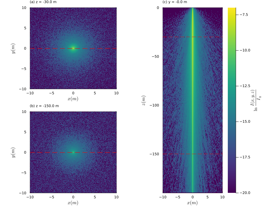

For a complete guide with details on each function and step, see the HydrOptics's Documentation.

Gallery

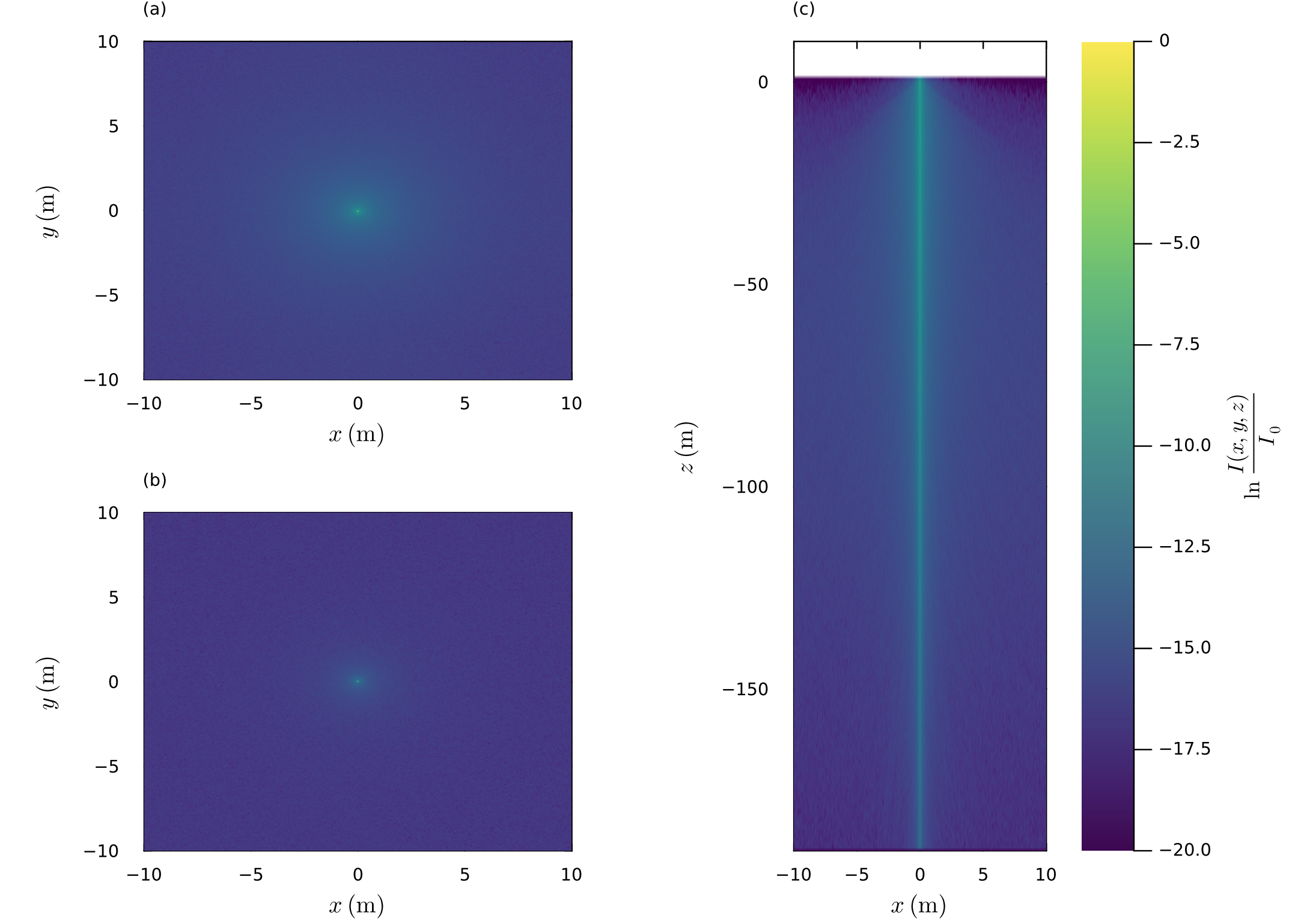
Simulation of $10^{8}$ Photons at the center of the flat surface. (a) irradiance field on the horizontal plane at $30\ \mathrm{m}$ depth. (b) irradiance field on the horizontal plane at $150\ \mathrm{m}$ depth. (c) irradiance field on the vertical plane at the center

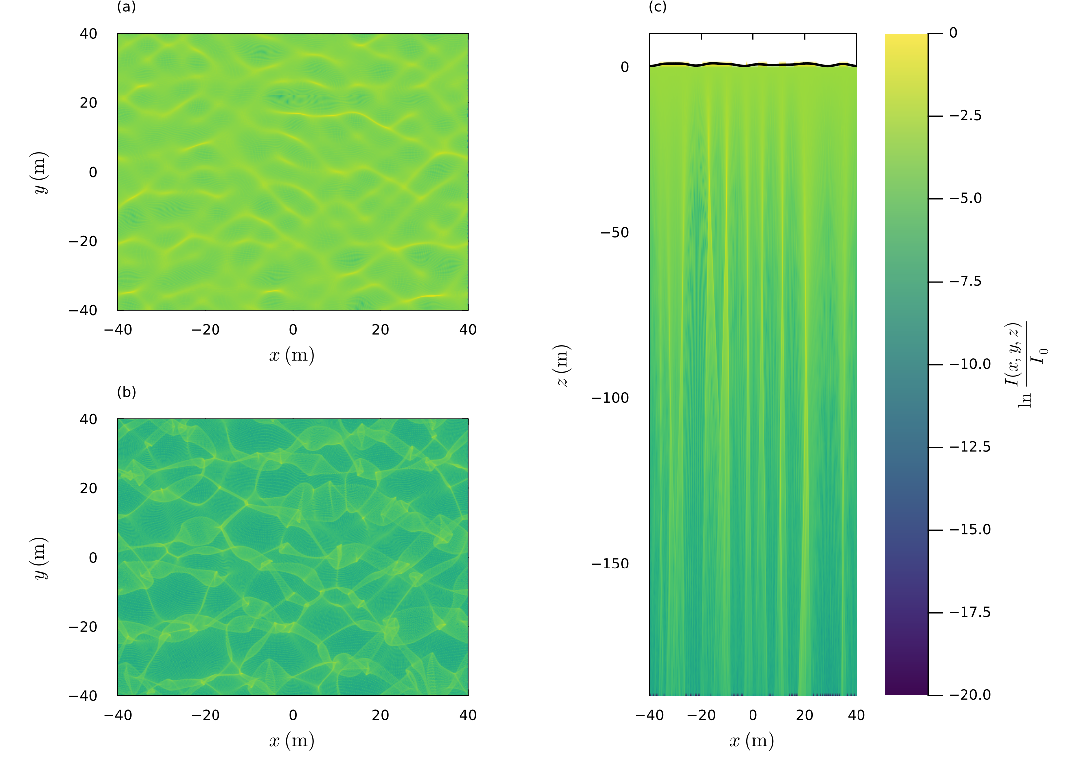
Simulation of 1000 Photons at the every grid point with observed surface elevation. (a) irradiance field on the horizontal plane at $30\ \mathrm{m}$ depth. (b) irradiance field on the horizontal plane at $150\ \mathrm{m}$ depth. (c) irradiance field on the vertical plane at the center.

Reference