Fundamental Principle of Monte Carlo simulation

The basis of Monte Carlo method lies in the idea that, if we know the probability of occurence of each separate event in a sequence of events, then we can determine the probability that the entire sequence of events will occur ^[1]. In the simulation of light within the water, each photon, after being transmitted into the water, travels in the medium, interacts with the molecule: absorb and scatter, and either being fully absorbed or reaches the measurement devices. With the multiple photons, we can determine the distribution of the light field.

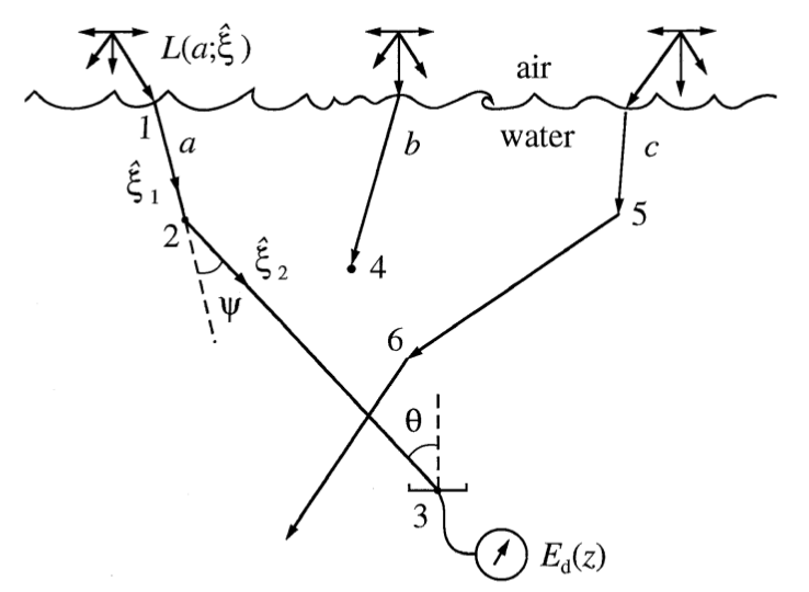
Illustration of three photons that are being emitted and travel inside the water medium^[1]

As mentioned above, the separate event that happens for each photon is consisted of travelling some distance in the medium, aborbing, and scattering. All of the events are determined by some probability. Hence, we define the probability distribution of a random number $p_{\Re}$^[1]

\[p_{\Re} (\Re) \equiv \begin{cases} 1 & \quad 0 \leq \Re \leq 1, \\ 0 & \quad \Re < 0 \cup \Re < 1. \end{cases}\]

The optical path length

After the photon's interaction with the medium or being transmitted into the water, we calculate for the distance the photon would travel before interact with the medium agian. The distance $r$ is defined by the equation below, when $c$ is the beam attenuated coefficient or the addition of absorbtance coefficient $a$ and scatterance coefficient $b$. ^[1]

\[r=-\frac{1}{c}\ln{\Re}\]

Sampling photon interaction type

Once, the photon travels for distance $r$, we, then, determine how it interacts with the medium: whether a photon will be absorbed or scattered. This can be done by drawing a random number $\Re$ and compare with the albedo of single scattering $\omega_{0} = \frac{b}{c}$, if $\Re\leq\omega_{0}$, the photon is being absorbed, and if $\Re\geq\omega_{0}$, the photon is being scattered. ^[1]

Sampling scattering direction

In the scattering event, we will calculate the scattering direction of the photon in the local spherical coordinate with azimuthal angle $\varphi$ and polar angle $\theta$. Azimuthal angle $\varphi$ is uniformly distribute between 0 and $2\pi$ hence, ^[1]

\[\varphi = 2\pi\Re\]

The angle between new trajectory and the direction before scattering $\theta$ is defined by the cumulative distribution, based on the experiment conducted by the Petzold(1972). ^[2]

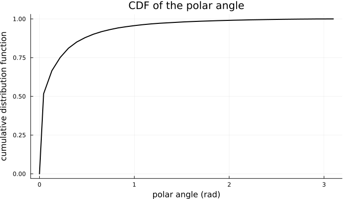
Cumulative Distribution Function of the polar angle or the angle between new trajectory and the direction before scattering $\theta$ based on the data from Kirk(1981)^[3]

Hence, we draw a random number $\Re$ and find the corresponding polar angle $\theta$ from the cumulative distribution function.

Reference